Infocus - Learning from the long end of the US term structure

LEARNING FROM THE LONG END OF THE US TERM STRUCTURE

Traditionally, market participants use the slope of the US term structure, as captured by the spread between 10-year and 3-months yields or between 10-year and 2-year yields, as an indicator of recession risks and prospects for the US economy. Few investors look further out along the term structure. In this issue of Infocus, EFG Chief Economist Stefan Gerlach extends the analysis to investigate the value of information contained in 30-year yields.

Executive summary

The slope of the US term structure is often used as an indicator of the likelihood of a recession and the outlook for growth. While the Fed typically looks at the spread between 10-year and 3-month rates, since different interest rates are generally strongly correlated, in practice it may not much matter precisely what spread is being used.

Few market participants look beyond 10-years. Yet, there is no reason to assume that longer yields are uninformative about the future path of the US economy. This issue of Infocus looks at nine Treasury yields with maturities from 3-months to 30-years and finds that longer dated yields contain information about future economic conditions that is not incorporated in traditional measures of the slope of the yield curve.

The analysis decomposes the term structure into three components that can be interpreted as capturing its level, slope and the difference between the slopes at the far and near ends. The latter factor is very strongly correlated with the spread between 30-year and 5-year yields minus the spread between 5-year and 3-month yields. Thus, it can be thought of as capturing information in the far end of the term structure that is not already incorporated in conventional measures of the slope of the term structure.

Not surprisingly, the empirical evidence presented shows that the slope factor contains information about future growth of industrial production at a horizon of about 12 months. However, the evidence also shows that the difference-in-slope factor is informative about industrial production growth but at longer horizons, starting about 24 months ahead, than the slope factor. It is also informative about changes in the slope factor with a lead of about 12 months. Neither factor is helpful for predicting future core inflation.

Looking at the actual forecasting performance of the slope and the difference-in-slope factors in the 1981-2020 period, it is clear that recessions were all preceded by both factors falling to very low levels.

For instance, the slope factor reached a minimum in November 2006, and the difference-in-slope factor in March 2005, well in advance of the recession of 2008 that was preceded by tensions in financial markets from Spring 2007 onward.

Similarly, the slope factor reached a minimum in August 2019, and the difference-in-slope factor in August 2018, well in advance of the recession of 2020 (which admittedly could not have been anticipated by financial markets).

However, while statistical evidence is clear, on a few occasions the difference-in-slope factor signalled a flattening of the term structure and a slowdown of growth, neither of which occurred. Of course, it is unsurprising that an indicator of recession risks at such long horizons is at times misleading. But while it may not be an entirely reliable indicator on its own, the evidence suggests that, in practice, it is best used as an early indicator that the term structure is about to become flatter or inverted and the risk of a decline in growth has risen.

Turning to the present situation, it is worth noting that both the slope factor and the difference-in-slope factor have steepened, implying that the market is pricing in continued economic recovery into 2021.

Introduction

There is ample evidence that the slope of the US interest rate term structure, or yield curve, contains information useful for forecasting the likelihood of a recession and the prospects for future growth in the US economy.¹ While the Fed typically looks at the spread between 10-year and 3-month rates – because that is the spread shown to have the best statistical ability to forecast recessions – market participants often look at other spreads, such as the spread between 2- and 10-year yields. Since different interest rates are typically strongly correlated with other interest rates of a similar maturity, in practice it may not much matter precisely what spread is being used.

But while much of the focus is on yields of up to 10 years, there is no reason to assume that longer yields are uninformative about the future path of the US economy. Furthermore, the same mechanism that may explain why the slope of the term structure predicts future economic conditions should be operative also in the case of longer yields.² Finally, the Fed’s database provides information on both 20- and 30-year constant maturity treasury yields.³ The punchline of the analysis below is that longer-dated yields contain information useful for forecasting future economic conditions that is not incorporated in traditional measures of the slope of the yield curve.

Additional technical explanations may be found in the blue frames.

The US term structure

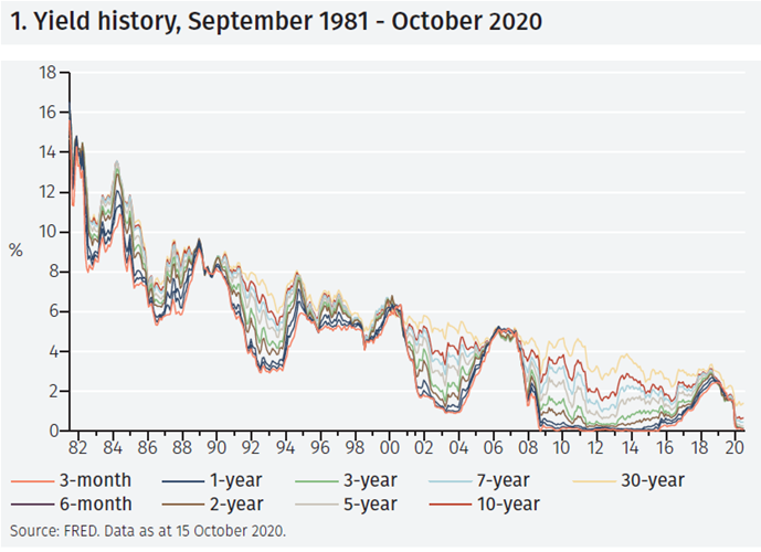
In this exercise, constant maturity Treasury yields for 3- and 6-month, 1-, 2- 3-, 5-, 7-, 10- and 30-year maturities are studied, with the focus on the information they may contain for core PCE inflation and the growth rate of industrial production. 

Figure 1 shows that the dominant movement in these yields over the period 1981 to 2020 is a gradual decline in their level from around 15-17% at the start of the sample to 0-1% at the end.

However, there are also large variations in the slope of the yield curve over this period. That is readily apparent following the recessions that started in 1981 and 1990 and during the global financial crisis in 2008-9 during which episodes the yield curve became steeply upward sloping.

It is hard to eyeball the data from the chart. To obtain a better sense of the information contained in these yields, principal component (PCs) analysis can be applied. This statistical technique creates a new set of time series that are linear combinations of the yields.

The principal components have two features. First, they are uncorrelated. Second, they are constructed to account for as much as possible of the variance of the data. Thus, the first PC is the linear combination of the yields that explains as much as possible of the overall variation in the yields studied. The second PC is constructed so as to explain as much as possible of the variation left unaccounted for by the first PC, and so on. With nine data series, nine PCs can be computed. However, the most interesting are typically the first few since by construction they explain the bulk of the variation of the data; below the first three are considered.

Three factors driving the term structure

Figure 2 overleaf shows the “factor loadings” for the PCs. These explain how they are constructed from the underlying yields.

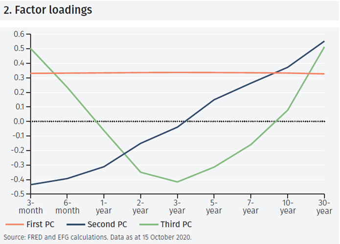
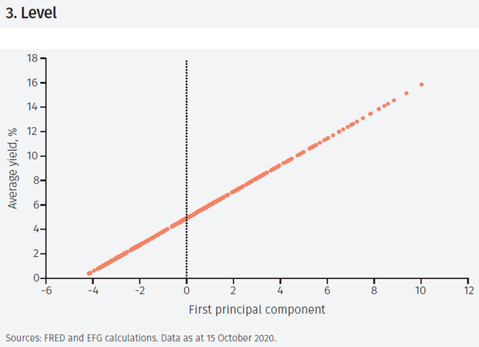
Interestingly, the factor loadings for the first PC, which explains about 97.8% of the variation of the yields in Figure 1, show that it is constituted of all the yields in roughly equal measure. Thus, it is (almost) an average of the yields studied. Indeed, as the scatter plot in Figure 3 shows, the correlation of the first PC and the cross-sectional average of the yields is almost unity. Thus, it is natural to think of the first PC as the level of the term structure.

The factor loadings of the second PC, which accounts for 2.0% of the variation of the data, are also shown in Figure 2. In this case the loadings are negative for short interest rates and positive for longer interest rates. This component thus reflects changes in the slope of the term structure.

To see this more clearly, Figure 4 shows a scatterplot of the second component against the 10-year to 3-month spread, which is the most commonly used measure of the slope of the term structure. As can be seen, the two series are extremely strongly correlated (the correlation coefficient is 98.6). The second PC can thus be thought of as the slope of the term structure.

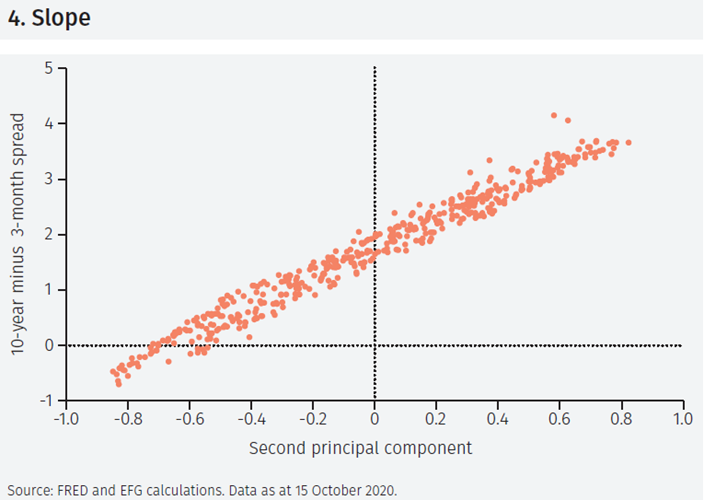
It is important to note that since different interest rates are strongly correlated, the second PC is also strongly correlated with other spreads. For instance, its correlation with the spread between 5-year and 3-month yields is 93.9.⁵ It is not surprising that different analysts prefer different measures of the slope of the term structure.

Finally, the factor loading for the third PC, which is constructed to explain as much as possible of the variation left over by the first and second PCs (and which accounts for 0.1% of the variation in the data), has a more complicated structure as Figure 2 shows: it has a positive weight on the longest and shortest yields and a negative weight on intermediate yields.

Perhaps surprisingly, it can be given an intuitive interpretation. To see this, Figure 5 shows a scatterplot of the third PC and the spread between 30-year and 5-year yields minus the spread between 5-year yields and 3-month yields. As can be seen, the two series are highly correlated (86.8).

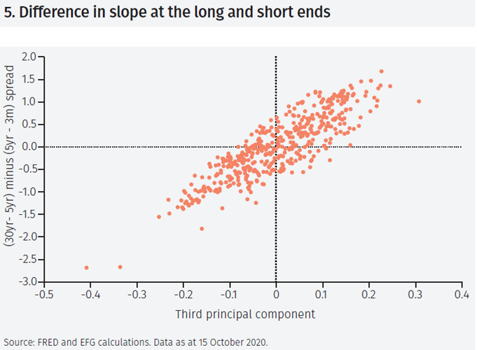
The third PC can therefore be thought of as the difference between slope of the term structure at the long end and at the short end. Intuitively, it contains the information in the term structure that is in addition to traditional measures of the slope. It goes without saying that this effect is likely to be quite delicate, may be hard to discern in the data, and it is not surprising that that it has not been studied much, if at all, in the literature.

The term structure and the macro economy

What information for economic activity and inflation do the level, slope and the difference in slope at the long and short ends of the term structure contain? This question can be addressed by including the three PC variables in a statistical (VAR) model, including also core PCE inflation and the growth rate over 12 months of industrial production.

While a market analyst would naturally think of these in terms of observed yields, the PCs are used in the modelling below since they are computed using a formal statistical procedure and use the information contained in all the nine yields.⁶

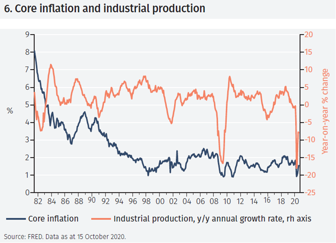
Figure 6 shows the evolution of inflation and the annual growth rate of industrial production in the sample period. The main feature of inflation is a gradual decline from above 8% in 1981 to below 2% in 2020. The figure also shows that industrial production growth declined far below zero during the financial crisis in 2008-9 and during the current Covid-19 pandemic. The growth rate of industrial production also turns negative during the recessions in the early 1980s, 1990s and 2000s.

Before turning to the results, a critical methodological issue must be addressed. In the statistical model, changes to the three PCs occur together. Not surprisingly, this is particularly so in the case of the shocks to the second and third PC, which capture the slope and the difference in slope between the longand short-ends of the term structure. That raises the question of how to distinguish between the effects of these two components or factors on inflation and industrial production. To do so, shocks to them must be “identified.”⁷

In real life, prior knowledge about how the world works is used to handle this situation.⁸ This is not possible here since no such prior knowledge is available. Instead, here it is assumed that the first PC is the most important driver of inflation and industrial production, followed by the second, and then the third, PCs.⁹ This assumption downplays the importance of the third PC in the estimates.

Figure 7 shows the main results of the statistical analysis. Consider first the graphs in the first column. These show that an increase in the level of the term structure has historically been associated with faster economic growth (first row) and higher core inflation (second row).

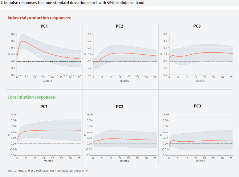
Since higher interest rates can be expected to slow the economy and reduce inflation pressures, these results may appear counterintuitive. However, financial prices are crucially influenced by expectations of future economic conditions. These results should be interpreted as bond yields rising as expectations of higher growth and inflation take hold.

The second column shows the effects of an increase in the slope of the term structure. As has been well documented, the upper graph shows that a steeper yield curve is associated with faster growth of industrial production. That effect is statistically significant after about 15 months. The lower graph shows that changes in the slope of the term structure contain no information about the future path of core inflation.

Finally, the third column shows the effect of a steepening of the far end of the term structure relative to the short end (that is, an increase in the difference-in-slope factor) which is the main focus of this exercise. Despite the fact that the third PC has been purged of any information contained in traditional measures of the slope the term structure, the upper graph shows that it has a significant effect on – or correctly predicts – faster growth of industrial production from about 24 months out. Thus, the information in the difference-in-slope factor provides a forewarning of changes in growth about 12 months before the slope factor.¹⁰ Furthermore, the numerical size of the effect is about as large as the effect of the slope factor: a one standard deviation shock raises the growth rate of industrial production in both cases by about 0.2%.

The lower graph shows that changes in the slope of the term structure do not contain information useful for forecasting inflation.

Discussion

The finding that both second and third principal components – or the slope factor and the difference-in-slope factor – contain information about the future path of industrial production raises the question of how they have evolved over the period studied.

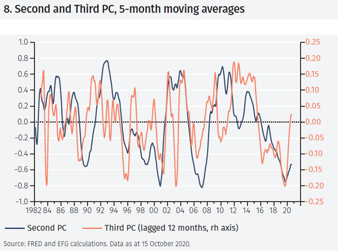
Figure 8 shows the two factors. Since the difference-inslope factor is volatile, 5-month averages have been used. Furthermore, the factor has been lagged by 12 months since it seems to predict industrial production about a year earlier than the second factor.

Discussion

Strikingly, the figure shows that both factors were negative before the 1990-91, 2001, 2007-2009 and the 2020 recessions. For instance, the slope factor reached a minimum in November 2006, and the difference-in-slope factor in March 2005, well in advance of the recession of 2008 that was preceded by tensions in financial markets from the spring 2007 onward.

Similarly, the slope factor reached a minimum in August 2019, and the difference-in-slope factor in August 2018, well in advance of the recession of 2020 (which admittedly could not have been anticipated by financial markets).

Closer inspection of the data shows that the third factor may occasionally give false alarms, as it declined to low levels in 1987, 1994 and 2002 without a subsequent slowing of the growth rate of industrial production. Of course, it is unsurprising that an indicator of recession risks at such long horizons is at times misleading. But while it may not be entirely reliable indicator on its own, the evidence suggests that, in practice, it is best used as an early indicator that the term structure is about to become flatter or inverted and the risk of a decline in growth has risen.

Turning to the present situation, it is notable that both have started to rise in recent months, implying that the market is pricing in continued economic recovery into 2021.

Conclusions

The main conclusions can be summarized as follows.

1. The information in the nine yields considered here can be summarised in three PCs that together account for almost all the variation in these yields (99.97%).

2. The first PC captures the average level of the term structure; the second its slope as captured by standard yield spreads; and the third the difference in slope between the long and short ends.

3. The first PC contains information about future growth and core inflation.

4. The second PC contains information about future growth at a horizon of about 12 months, but no information about future inflation.

5. The third PC (which by construction is unrelated to the second PC) contains information about future growth about 24 months ahead and of the future slope of the term structure about 12 months ahead. It contains no information about future core inflation.

6. The recessions in the period studied were all preceded by both the second and third PCs falling to very low values. However, the third PC signalled a few slowdowns of growth that did not occur. Thus, it needs to be interpreted with care.

Footnotes

1 The website of the New York Fed contains references to a number of studies on the ability of the term structure to forecast recessions: https://www.newyorkfed.org/research/capital_markets/ycfaq.html#/

2 That is, the expectations hypothesis, which states that long yields depend on the expected path of short rates, plus potentially a risk premium that is constant but may vary with maturity. This theory implies that as market participants come to expect an economic slowdown or recession, they also expect that the central bank will cut interest rates in the future, leading long yields to decline relative to short yields.

3 Data on 20-year yields are missing for the period January 1987 to September 1993.

4 The principal components can be thought of as weighted averages of the individual series, with the weights related to the factor loadings.

5 In the 1980s, the long end of the term structure was often almost flat while the short end was rather steep. Over time, the two slopes have converged in trend wise fashion. This trend is accounted for Figure 5. Without this adjustment the correlation is 55.4.

6 The VAR(2) model is estimated over the sample November 1981 to August 2020.

7 While the principal components are uncorrelated, the residuals in the VAR models are not: the correlation between the residuals in the equations for the slope and the change of the slope of the term structure is -0.40.

8 For instance, the fact that umbrellas are only used when it rains is attributed to rainfall leading people to use their umbrellas, not to the use of umbrellas causing rainfall.

9 That is, they are “ordered” in this way when the Choleski factorisation is used.

10 The complete set of results (not included) shows that a rise in the long end of the term structure furthermore leads to a gradual steeping of the term structure that peaks after about 12 months.

Important Information

The value of investments and the income derived from them can fall as well as rise, and past performance is no indicator of future performance. Investment products may be subject to investment risks involving, but not limited to, possible loss of all or part of the principal invested.

This document does not constitute and shall not be construed as a prospectus, advertisement, public offering or placement of, nor a recommendation to buy, sell, hold or solicit, any investment, security, other financial instrument or other product or service. It is not intended to be a final representation of the terms and conditions of any investment, security, other financial instrument or other product or service. This document is for general information only and is not intended as investment advice or any other specific recommendation as to any particular course of action or inaction. The information in this document does not take into account the specific investment objectives, financial situation or particular needs of the recipient. You should seek your own professional advice suitable to your particular circumstances prior to making any investment or if you are in doubt as to the information in this document.

Although information in this document has been obtained from sources believed to be reliable, no member of the EFG group represents or warrants its accuracy, and such information may be incomplete or condensed. Any opinions in this document are subject to change without notice. This document may contain personal opinions which do not necessarily reflect the position of any member of the EFG group. To the fullest extent permissible by law, no member of the EFG group shall be responsible for the consequences of any errors or omissions herein, or reliance upon any opinion or statement contained herein, and each member of the EFG group expressly disclaims any liability, including (without limitation) liability for incidental or consequential damages, arising from the same or resulting from any action or inaction on the part of the recipient in reliance on this document.

The availability of this document in any jurisdiction or country may be contrary to local law or regulation and persons who come into possession of this document should inform themselves of and observe any restrictions. This document may not be reproduced, disclosed or distributed (in whole or in part) to any other person without prior written permission from an authorised member of the EFG group.

This document has been produced by EFG Asset Management (UK) Limited for use by the EFG group and the worldwide subsidiaries and affiliates within the EFG group. EFG Asset Management (UK) Limited is authorised and regulated by the UK Financial Conduct Authority, registered no. 7389746. Registered address: EFG Asset Management (UK) Limited, Leconfield House, Curzon Street, London W1J 5JB, United Kingdom, telephone +44 (0)20 7491 9111.

Please use the button below to download the full article.